• Welcome to the MHE Blog. We'll use this space to post corrections and comments and to address any questions you might have about the material in Mostly Harmless Econometrics. We especially welcome questions that are likely to be of interest to other readers. The econometric universe is infinite and expanding, so we ask that questions be brief and relate to material in the book. Here is an example:
    "In Section 8.2.3, (on page 319), you suggest that 42 clusters is enough for the usual cluster variance formula to be fairly accurate. Is that a joke, or do you really think so?"
    To which we'd reply: "Yes."

MHE at 12000 feet

Andrea Ichino takes the RD message to new heights (specifically, to Cime Nere in Italian, as Andrea would like it; Hintere Schwarze in German – the peak straddles the Italian-Austrian border 3624m)

MHE RD shirts worn by the entire team, though as far as I know they were not planning to jump local discontinuities

Published | Tagged | Leave a comment

keep those corrections coming!

our corrected printing notwithstanding, we certainly didn’t catch them all . . .

here’s a few more from Aron “eagle-eye” Tobias at Yale:

The book is really great but I need not tell you that since you
probably know that already. What I would like to share with you is
some possible typos (all are really minor, though):

 * pp. 123--125. There are multiple minor inconsistencies between
figures reported in table 4.1.1 and the text. On p. 123, it is claimed
that "[i]n both cases, the estimated return to schooling is around
.075[,]" whereas the figures reported in columns 1 and 2 in table
4.1.1 are .071 and .067, respectively. Similarly, the assertion that
"[t]hese estimates range from .10 to .11[,]" appears on the same page
but columns 3 and 4 in the table indicate .102 and .130, respectively.
In addition, on p. 125, "...the standard error declines from .019 to
.016 as we move from column 6 to column 7" but the table indicates
that it declines from .020 to .016, presumably because of the figures
in the table and the text being rounded differently.

* p. 130 "The Wald estimate of the effect of military service on 1981
earnings, reported in column 4[;]" in fact, they are reported in
column 5.


* p. 131. By "...defined using the 1952 lottery cutoff 95..." you
probably mean the 1972 lottery.

* p. 132. "...a multiple third birth increases this proportion to 1"
should be "...a multiple second birth [i.e. a second birth in which
the second and third babies are twin-born] increases this proportion
to 1."

* p. 351. The Hausman (2001) reference has the title of the journal
wrong (Journal of Econometric Perspectives should be The Journal of
Economic Perspectives).

I apologize in advance if any of my claims turns out to be erroneous.

I remain your faithful reader,
Aron Tobias
Ph.D. Student, Department of Economics, Yale University

thanks Aron
All I can say is, how come Steve didn't catch these last year?!


JA
Published | Tagged | Leave a comment

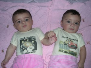
Twin Econometricians!

Here’s a pair of the cutest econometricians we have ever seen, helpin’ their mama (Daniela Vuri) run regressions every day

Martina and Lavinia . . . Mostly Harmless

Published | Tagged , | Leave a comment

Lagged Dependent Variables with Random Effects

Henrik Lindemann would like to come back to our advice not to use fixed effects and
a lagged dependent variable at the same time (see chapter 5.3/5.4 as
well as your blog entry of October 6, 2009).
Is it possible to use at least a random effects model in case I decide
to use the lagged variable or does the latter always require a pooled
regression?  In other words: Is it somehow possible to take the data
structure into account (the panel consists of 30 OECD countries)?
Good question Henrik. If you have, say, random country effects in a country panel then the lagged dependent variable will be correlated with the random effect in your error term. So you can't estimate that model by OLS and get what you want. This is a lot like the complications that arise in panel models with fixed effects and serial correlation - they get messy and hard to identify, perhaps even harmful. Random effects are just as troubling as fixed effects in the lagged dependent variable case. Better to just add more lags and hope this soaks up any serial correlation that messes up inference. Otherwise, it's oil and water. JA
Published | Tagged , | Leave a comment

Principals of principal stratification

Mike Sconces asks:

Question: I have questions about "bad control" (BC) (Section 3.2.3, p.
64). Your prescription is to leave the BC out of the model, or else to
have strong theory for leaving it in. In the stats literature, there
is discussion of "principal stratification" (PS). Let w_0i, w_1i be
the potential outcome of a mediator variable (following the notation
on p. 65) for individual i. The idea of PS is to divide the sample
into, e.g., {i: w_0i = w_1i} and {i: w_0i != w_1i}. These strata are
generally unobservable, but we could otherwise use them as
pre-treatment covariates. Some stats papers argue that the LATE relies
on a special case of PS, where the sample is divided into those whose
treatment status is affected by the instrument, and those whose
treatment status is not. Here, the treatment would be a BC (in the
reduced form, I suppose...?). So why doesn't PS make us more hopeful
about BC? Also, given random treatment, why can't we just instrument
the BC, since it's just another endogenous variable?


Published | Tagged | 1 Comment

Heteroskedasticity and Standard Errors – big and small

From Winston Lin:

Comment: On p. 307, you write that robust standard errors “can be smaller than conventional standard errors for two reasons: the small sample bias we have discussed and their higher sampling variance.” A third reason is that heteroskedasticity can make the conventional s.e. upward-biased. In your Monte Carlo study, heteroskedasticity makes the conventional s.e. downward-biased, because the smaller group (the treatment group) has the larger variance. If you instead choose sigma > 1 (so the control group has the larger variance), the conventional s.e. will be upward-biased (because when we pool the residuals, we overestimate the variance of the treatment group mean more than we underestimate the variance of the control group mean).   I’m sure you’re aware of this, but it might be worth noting explicitly, to avoid giving the impression that robust s.e.’s “should” be larger than old-fashioned s.e.’s.

Thanks for writing such a helpful, insightful, and fun book!

Thanks for this insight, Winston.

Indeed, in writing section 8.1 on robust standard errors we have not really appreciated the fact that conventional standard errors may be either too small or too big when  there is heteroskedasticity.  Winston is right that it can go both ways.  The attached note describes the mechanics, and gives conditions  for the direction of the bias.  Basically, conventional standard errors are too big whenever covariate values far from the mean of the covariate distribution are associated with lower variance residuals (so small residuals for small and big values of x, and large residuals in the middle of the x range).  We think this is empirically not the common case but it might happen.  The leading case is probably that residual variance goes up with the value of x (true for example in the returns to schooling example: earnings are more variable for those with more schooling).  In this case, conventional standard errors will tend to be “about right” or too small as the discussion in 8.1 suggests.

JSP

Published | | Leave a comment

ex post T and C for DD

Mel asks:

Question: My understanding of a difference in difference model is that
the two groups should exist before a policy takes affect (e.g. two
states, companies, school districts).  I was studying the impact of a
policy on an outcome where the two groups did not exist until the
policy went into effect and everyone was eligible for the policy all
at once.  There was no staggered implementation.  Because of this I
thought to use a lagged dependent variable model to study the impact
of the taking advantage of the new program offered through the policy.
 DVt1= Program + DVt-1 + error.  This model would at least allow me to
control for the separate groups in time two.  I recently saw someone
publish on my topic but they used a difference in difference model.
They assigned the program status which in reality could only occur in
t1 after the policy went into affect to the same people in t-1 when
the program did not exist. I did not think this was correct, thus I am
writing for clarification.

thanks for your question Mel

check out the classic training evals by Ashenfelter (1978) and Ashenfelter
and Card (1985).  They compare pre and post for trainees and controls.
They don't know who is a trainee until "period 2." Once training status
is known, however, it's easy to reach back (in a panel) for pre-treatment
obs for both groups.  

Is this a credible identification strategy?
Probably not as good as being able to make an ex ante T and C distinction,
but sometimes ok.
well, when is this ok . . .
Check out the originals and find out!  These classics do a great job of
explaining why and when this sort of DD makes sense . . .

JA
Published | Tagged , | Leave a comment

The t and the p for just-ID will never surprise thee

My people always say that before embarking on a difficult empirical project.  A free t-shirt to the first poster who translates.

JA

Published | Tagged , | 8 Comments

Regression Is Matching (one more way; with discussion!)

Pat Kline has a nifty new interpretation of the old Blinder-Oaxaca regression estimator for two-group comparisons (in this case, applied to treatment effects in a selection-on-observables setup) . . .  It’s a matching estimator, of course!

Here’s the version we saw at ASSA in Denver, niftier than ever!

and my discussion, which is pretty good too . . . JA

Published | Tagged , | Leave a comment

Kindle KAOS

A few disappointed readers have commented that the kindle version of MHE suuu . . . is not so hot.  Math font KAOS, Mr. Smart! (with type set by Shtarker, among other unforgivable glitches.) But ebook aficianados don’t dispair, just install one of Amazon’s free reading apps and read glitch-free on the hardware of your choice (iphone, windows PC, Mac, Blackberry, Android – anything but the Kindle reader! I tried it on my Mac – nice VIV!

JA

Published | Tagged , | 1 Comment